But where on Earth is my eye candy?
Now that we have some procedure and results, we would like to be able to show this to the outside world (and to be honest, some graphical results would also help getting confidence in results).
The additional task to do so is really minimal. What we need to do is simply to put back those numerical results into the ANSYS database so that we can use all the conventional post-processing capabilities. This can be made using the appropriate POST1 commands, essentially: DNSOL. And, while we are at it, why not do a hardcopy to an image file? Here is the corresponding input.
… User should place all nodes with non-prescribed temperatures in a component named MyNodeComponent

… First, convert Eigenvectors from solver to BCS ordering
! Conversion needed
*SMAT,Nod2Bcs,D,IMPORT,FULL,Jobname.full,NOD2BCS
*MULT,Nod2Bcs,TRAN,MatPhi,,MatPhi

! Then, read in mapping vector to convert to user ordering
*VEC,MapForward,I,IMPORT,FULL,Jobname.full,FORWARD

! Put the results in ANSYS database
/POST1
*do,ind_mode,1,NRM
	cmsel,s,MyNodeComponent
	curr_node=0
	*do,i,1,ndinqr(0,13)
		curr_node=ndnext(curr_node)
		curr_temp=MatPhi(MapForward(curr_node),ind_mode)
		dnsol,curr_node,TEMP,,curr_temp
	*enddo

	Tau=1/(2*3.14*EiV(ind_mode))**2

	To=NINT(Tau*10)/10 ! compress to 1 digit after comma
	/title,Mode #%ind_mode% - Tau=%To%s
	plnsol,temp
     ! Hardcopy to BMP file
     /image,SAVE,JobName_Mode%ind_mode%,bmp
*enddo
This way, modes can be displayed, or even written to a conventional .RTH file (using RAPPND), and used as any regular ANSYS solver result.
Nice, but an actual example wouldn’t hurt, would it?
Now you may wonder what the results look like in reality. To remain within the field of precision engineering, let’s use a support structure typically designed for high-stability positioning. From a structural point of view, it must have a high dynamic stiffness and a low total mass so that a Delta shaped bracket is appropriate. Since we want the system to rapidly evacuate any heat load, we choose aluminum as candidate material. We do know from first principles that any applied disturbance will exponentially vanish and the system will go back to equilibrium state. Now, what will be the time constants of this decay?
For the sake of simplicity we restrict the analysis to a highly simplified, 2D model of such a support. PLANE55 elements are used to model the structural part while the heat sink is accounted for using SURF151. Boundary conditions are enforced using an extra node.
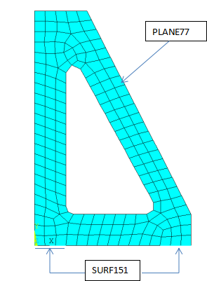
After applying boundary conditions, we execute the modal solution to obtain say – the first 8 modes.
| Index | Tau [s] | Comment |
|---|---|---|
| 1 | 535.9 | Quasi-uniform temperature field (i.e. equivalent of a “rigid body” mode) |
| 2 | 32.1 | 1st order (one wavelength along perimeter) |
| 3 | 23.8 | 1st order (one wavelength along perimeter) |
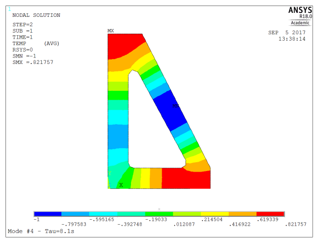
| 4 | 8.1 | 2nd order (two wavelengths along perimeter) |
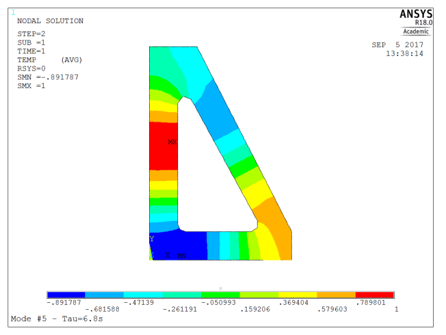
| 5 | 6.8 | 2nd order (two wavelengths along perimeter) |
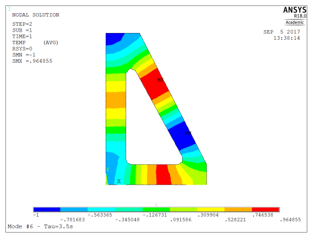
| 6 | 3.5 | 3rd order (three wavelengths along perimeter) |
| 7 | 3.1 | 3rd order (three wavelengths along perimeter) |
| 8 | 2.2 | 4thorder (four wavelengths along perimeter) |
The output (not repeated here) is strictly the same as the one a standard modal analysis, except for the two additional lines at the end of the solving sequence.
Allocate a [8] Vector : EIV
Allocate a [227][8] Dense Matrix : MatPhi
Instead of writing the solution to the result file, one vector and one matrice have been added to the ANSYS workspace. Please note that the solution has 227 DOFs whereas the entire problem has 228 DOFs. This is the consequence of having introduced the boundary conditions as an enforced temperature on a node, which DOF is therefore removed from the DOF set to be obtained by the solver.
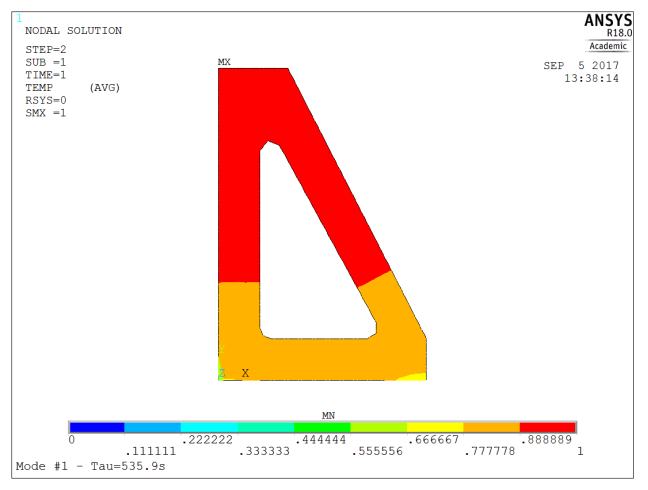 | 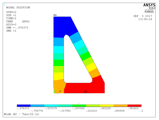 |
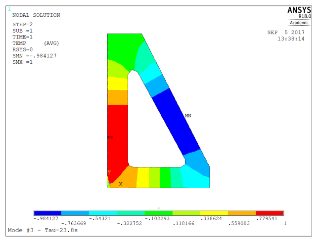 |  |
 |  |
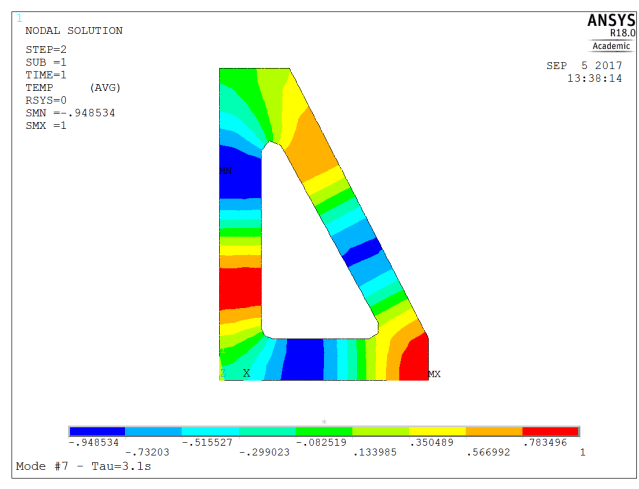 | 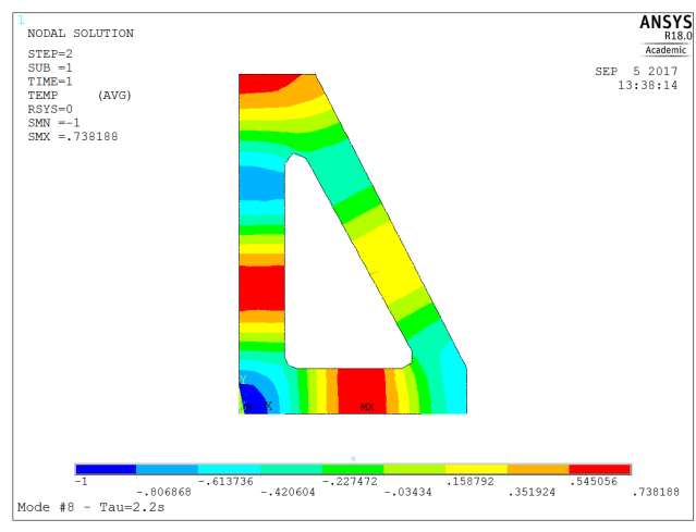 |
Now, this information tells us that a thermal imbalance between the bottom and top the bracket will decay with a time constant of about 32s. In order to come to equilibrium with its surroundings, the time constant would be about 500s, so about 20 minutes (2.3 x time constant) will be required so to reduce the temperature offset to 10% of its initial value.
Also, we might want to use the modal shapes information to decide which locations are best suited to capture the entire temperature field on the structure. Without knowledge of the excitation source, one straightforward way to do so is to retain for each mode the node that has the largest amplitude. This is made even easier in this situation, since we have normalized each mode to have unit maximum amplitude we just need to select nodes having modal amplitude equal to 1 (or -1). On the figure below, each temperature sensor location is marked with a ‘TSm’ label where m is the mode index.
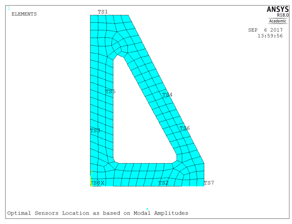
Doing so, we reach a pretty satisfactory distribution for the sensors locations, completely consistent with intuition. In numerical terms, we can also check that the modal matrix restricted to the selected DOFs, has an excellent condition number. But there are many other things we could do starting from this. For example, with additional information, such as the location and the frequency content of the temperature fluctuations, one could further restrict the set of needed temperature sensors by running a dummy transient analysis and choosing locations where the correlation between sensors readings is as low as possible (using *MOPER,,,CORR). Even better, one can estimate the thermally induced displacements and select locations best suited to build an empirical model (typically using AR or ARMA), allowing one to predict structural displacements induced by temperature fluctuations using just a couple of sensors. This in turn can be used to select control strategies, check modal controllability… all within ANSYS
