Some concrete application wouldn’t hurt, would it?
Now that we have a new tool, we would like to toy around with it (and don’t even try denying it, if you have continued to read until this point, I know you do).
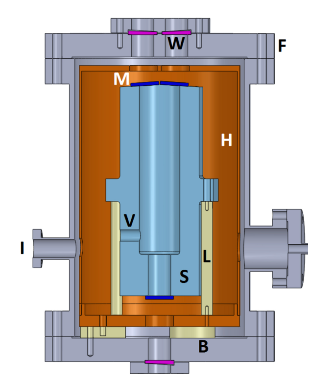
As an example, let’s consider the optical reference cavity depicted here. It is taken from reference [2], and basically aimed for IR interferometry. In terms of a thermal system, it is a “box in a box in a box”. The first one (blue colored) is the optical cavity, which we aim at keeping unaffected by the inevitable temperature fluctuations of this cruel world. It is contained in a second box (a thermal shield, copper colored), which itself is contained in a third box (the vacuum chamber, gray colored).
Now to introduce it’s usage: Let’s say it is an enclosure with highly reflective boundaries (mirrors “M”) onto which photons will bounce back and forth a great number of times, until only particular wavelengths subsist (the ones for which the return flight corresponds to a half integer multiple of the cavity length). This very regular phenomenon is used to narrow down the bandwidth of laser sources, and the beauty of it is that there are little intrinsic limits to the stabilization performance, except one: thermal drifts. Actually, in the realm of physics, optical sources with 10-14 to 10-16 stability rates (i.e. strain rate of 10-14 to 10-16 s-1) are not uncommon. Provided that the spacer (V) is made of state of the art material like Zerodur (Coefficient of Thermal Expansion of about 10-8/deg), we are looking at thermal stabilities of the order of 10-6 to 10-8degC/s. One micro degC is surely not a common engineering unit but in our case, it becomes the allowable value!
Every effort was made to limit heat propagation from the exterior to the interior of the system, using low conductivity mechanical supports and radiation shielding. But, how do we know that our fine-looking thermal enclosure is appropriate to reach say a 1µdegC/s or even 0.01degC/s stability?
First, we build the model just like for any other regular thermal analysis.
Note that, for cases like this one where radiation needs to be accounted for, then only the radiation matrix (aka /AUX12) method can be used (see here for details https://www.padtinc.com/blog/wp-content/uploads/oldblog/PADT_TheFocus_53.pdf ). Also, be aware that during the generation of the capacitance matrix, a dummy radiation superelement (MATRIX51) with near-zero terms must be used (most simply by specifying a tiny value for the Stefan Boltzmann constant, as input via the STEF command).
Also, in perspective of easier interpretation of results, we introduce 3 additional (“master”) nodes, at key locations (spacer, upper and lower mirrors). Their temperature is calculated by arithmetically averaging the temperature at selected sets of nodes. This is done by using Coupling Equations (CE command) generated using a *DO loop. Basically, we wish that the following relationship is respected:

By doing this we access the average temperature of subsets of the model. In one sense, this is the thermal equivalent of using the RBE3 command (another NASTRAN command by the way, and yes, more hiss is coming. Have a ball!). A bit of warning here, including many (1000+) nodes in a coupling equation might significantly increase the solver wavefront, and hence peak memory usage, so you might want to reduce the spatial sampling.
Then, to generate conductivity (MatK) and capacitance (MatC) matrices, we run two transient dummy analyses with either conductivity or capacity effects activated. To avoid any possible confusion, we change the file name each time (Run_Thermal_MatK and Run_Thermal_MatC), so that matrices are stored into separate .FULL files. Note that, although excitation is not needed at that point, boundary conditions are already required, hence we set . Then, we add the excitation by enforcing a unit temperature at the outer boundary of the system (where temperature sensors are allowed), while keeping the rest at null temperature, and run a third one step dummy transient analysis (Run_Thermal_VecF).
We exit ANSYS (though it’s not required) and start a new run, beginning with importing the corresponding matrices/vector. Please note that the FE model is not strictly required anymore, except if display or structural capabilities must be used.
The output window confirming that everything is fine should read as follows.
Import Data From File Run_Thermal_MatK (Format=MAT)

  Import Data From File Run_Thermal_MatC (Format=MAT)

  Import Data From File Run_Thermal_VecF (Format=MAT)
  Copy the matrix VECF_REAL to the matrix VECF

  Import Data From File Run_Thermal.full (Format=FULL)
  Import the internal node ordering to boundary condition mapping

  Import Data From File Run_Thermal.full (Format=FULL)

Copy the matrix VECF to the matrix XBCS
Then we begin solving for our unknowns (as always with *DO, only the first iteration is shown):
…
*DO LOOP ON PARAMETER= IND_F FROM  1.0000     TO  30.000     BY  1.0000

 PARAMETER CURR_F =    0.1000000000

 PARAMETER W =    0.7272199074E-05
  Copy the matrix MATC to the matrix MATA

 *AXP COMMAND : ADD MATK CONTRIBUTION TO MATA MATRIX
  MYBCSSOLVER Engine : Use the BCS solver applied to the MATA matrix
 SPARSE MATRIX DIRECT SOLVER.
   Number of equations =        55891,     Maximum wavefront =    3815
  Memory allocated for solver =        1802.041 MB
  Memory required for in-core =         533.459 MB
  Memory required for out-of-core =     173.765 MB

Launch the numerical factorization of MYBCSSOLVER
 Sparse solver maximum pivot= 86421.2482 at eqn 20335.
 Sparse solver minimum pivot= 0.261744844 at eqn 17740.
 Sparse solver minimum pivot in absolute value= 0.261744844 at eqn
 17740.
  Solve Using Solver MYBCSSOLVER

  Allocate a [55891][1] Dense Matrix : TBCS
  Nrm VECF[0] = 2.944604E+004
  Nrm TBCS[0] = 2.335645E+002
  Copy the matrix TBCS to the matrix TBCSR
  Copy the matrix TBCS to the matrix TBCSI
  Multiply : NOD2BCS(T) by TBCSR -> TINTR
  Multiply : NOD2BCS(T) by TBCSI -> TINTI
In the present case, using an Intel Xeon CPU E5-1620@3.50GHz processor, the elapsed time for each frequency is about 6s for a 55kDOF problem, so that when 30 frequency points are used, the total run time is about 3 minutes. It is not difficult to see why such an approach is largely more efficient compared to a time domain one (which would probably not solve anyway due to disk space limitations).
Now we might want to have a look at the temperature fields. To do so using the General Postprocessor (POST1), we need to write the results into a thermal (.RTH) file. But, contrary to the Modal Analysis, results here are complex quantities, which are not supported by POST1. Hence, we need to write real and imaginary parts into separate files. We do that by creating (copying) the result file created during the generation pass, changing the job file name, resetting the case point to the beginning (SET/LCDEF) and appending the results (RAPPND). The corresponding code is given here for the real part of the solution:
/sys,copy RUN_THERMAL.RTH RUN_FRF_THERMAL_REAL.RTH
/filnam,RUN_FRF_THERMAL_REAL,OFF
! Store into .RTH file
/POST1
set,first
lcdef,erase

! STORE REAL PART
*do,ind_F,1,F_nb_steps
 curr_F=F_table(ind_F)
  ! Store complete solution
  *do,ind_node,1,nb_nd_res
	curr_node=NodeList(ind_node)
	dnsol,curr_node,TEMP,,TsolMatR(ind_F,ind_node)
   *enddo
   rappnd,1,curr_F
*enddo
Naturally, one should repeat that same operation for the imaginary part of the solution.
Once we are done, we can enjoy colorful images.
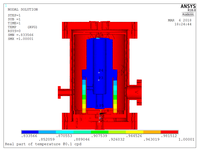
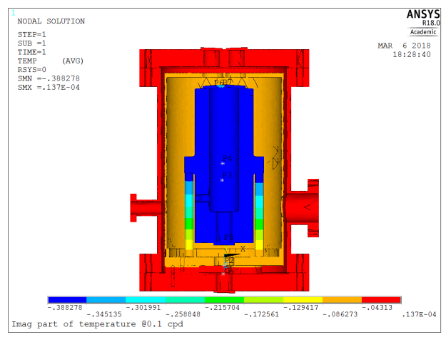
For very slow temperature transients, we expect the temperature to be nearly homogeneous, and in-phase with the excitation. Let’s have a look at the results for a 0.1cpd (10 days period) excitation frequency.
Results are indeed consistent with engineering judgment:
- Amplitude in the core of the system is about 90% (
 ) of that applied at the outer boundary
 - Phase lag is small (
 °)
°)
For faster fluctuations, response amplitudes should drop sharply, and this is actually the case.
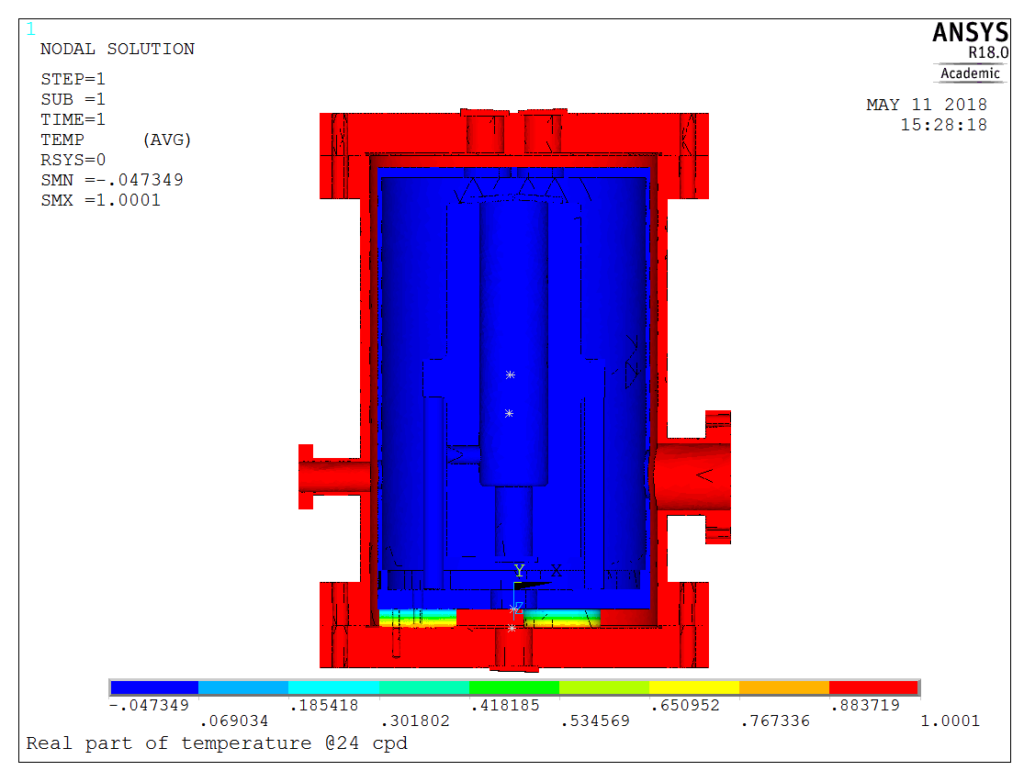
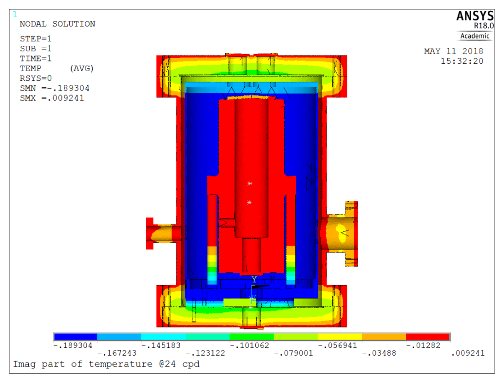
As an example, for 24 cpd fluctuation (1 hour period), the results are as follows:
At this frequency, the transfer efficiency is less than 5%, and the graphical method becomes impractical. This is where the text output comes to help. What we need to do is plotting the response amplitude vs frequency. In this example, we plot the temperature of the spacer, the lower and the upper mirrors, the three of them making the optically active part of the system. From this graph, it is apparent that although the three of them are connected, their behavior is not always identical, and that depending on the frequency, various effects dominate (radiation/diffusion). Actually, the response amplitude on the spacer @24 cpd is slightly below 0.3% of the excitation amplitude!
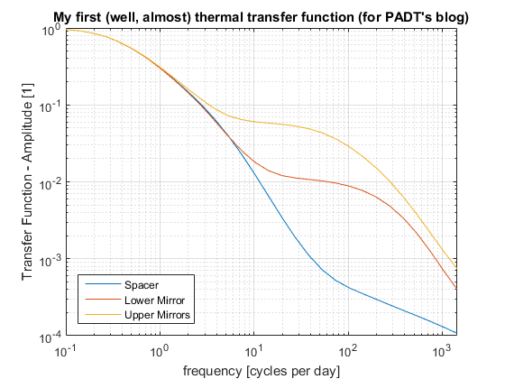
Returning to our original question (“how does temperature fluctuations propagate into the inner cavity”), we see that the answer is both location and frequency dependent. At 24cpd, there is a factor of 10 between response amplitude of the upper mirrors compared to the spacer.
Hence, in case a control system is used, it must take care of the long-period fluctuations (frequencies below 3 cycles per day, i.e. periods longer than 8 hours), but should be restricted to that bandwidth. The shorter temperature fluctuations will be taken care of passively by the inertia of the system, with a reduction factor above 103 for temperature fluctuations shorter than 1 minute.
Actually, it would even be detrimental to attempt controlling fluctuations shorter than 8 hours. This is clearly visible on the phase plot, as seen below:
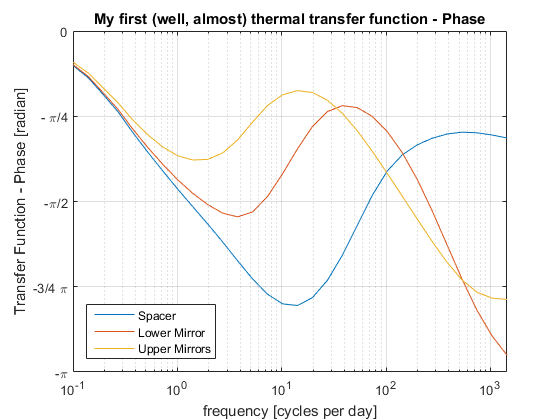
Starting from 1 cycle per day, the phase response of the various components becomes different. Attempting to stabilize one would result in de-stabilizing the others.
Obviously, the next step is to feed this information into a structural analysis to derive the thermal structural response of the system, but this is left as an exercise to the reader J. I don’t know about you but if you have read this post until here (I have already written 3000+ words) you probably want to call it a day!

