Compression using SVD: sample usage
Remember the aluminum bracket-shaped support we used in Episode 1 to illustrate Thermal Modal Analysis? It wouldn’t hurt to use it again, since it can be handy to demonstrate the similarities and differences between the POD basis (i.e. the left singular vectors) and classical Normal modes
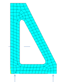
Let’s assume our bracket is submitted to a random temperature at its base, and see how its thermal response can be compressed using SVD.
For ease of understanding, this temperature signal is filtered white noise, using a order-1 low pass filter with time constant equal to 30s. Its amplitude is adjusted so that its standard deviation is unity (i.e. 1K RMS). We apply this temperature signal as a boundary conditions at the bracket support, and estimate temperature fields every second, for a total duration of 1000s, hence 1000 snapshots. In terms of space-wise discretisation, let’s first use the most simple element we have i.e. the good old PLANE55 (linear, i.e. 4 nodes element).
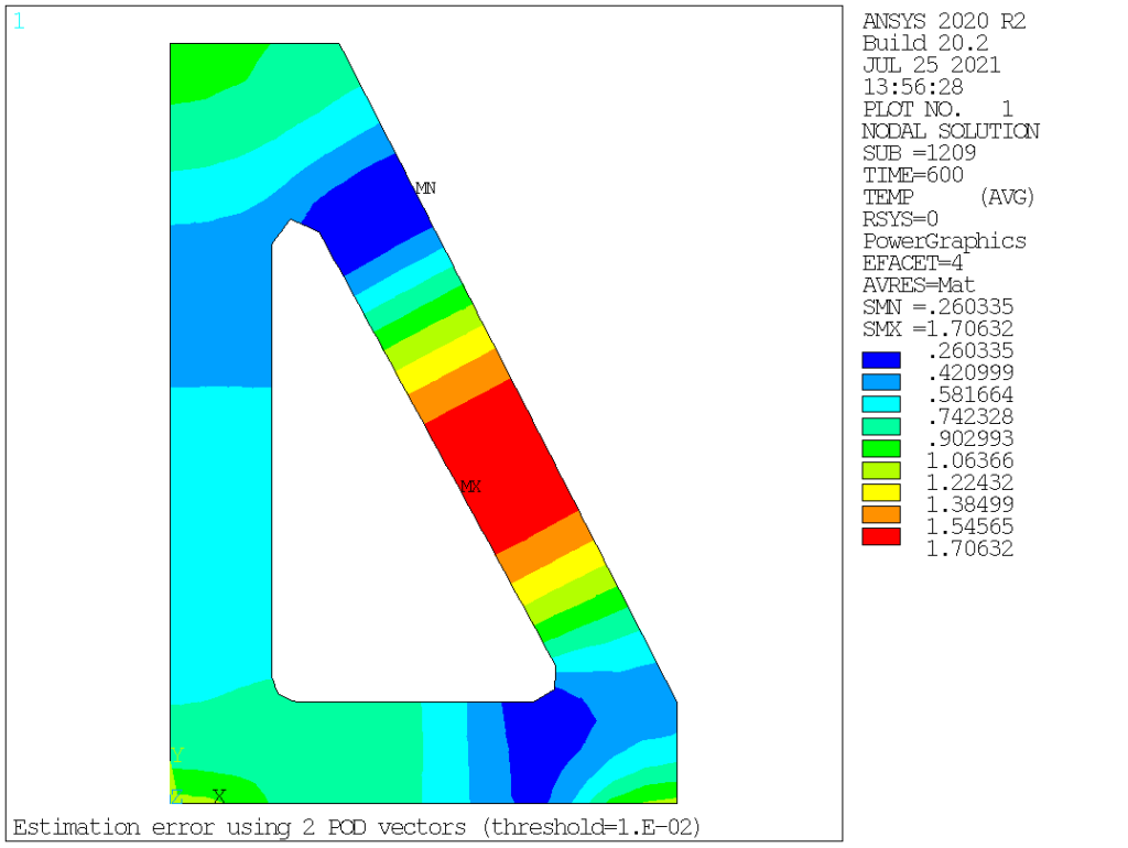
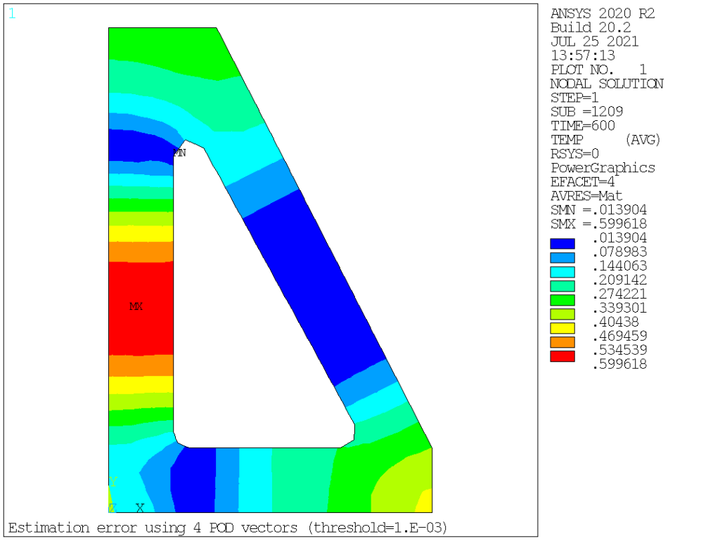
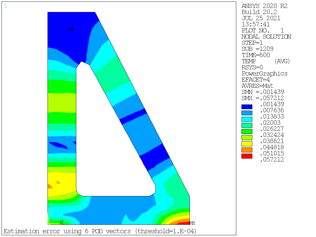
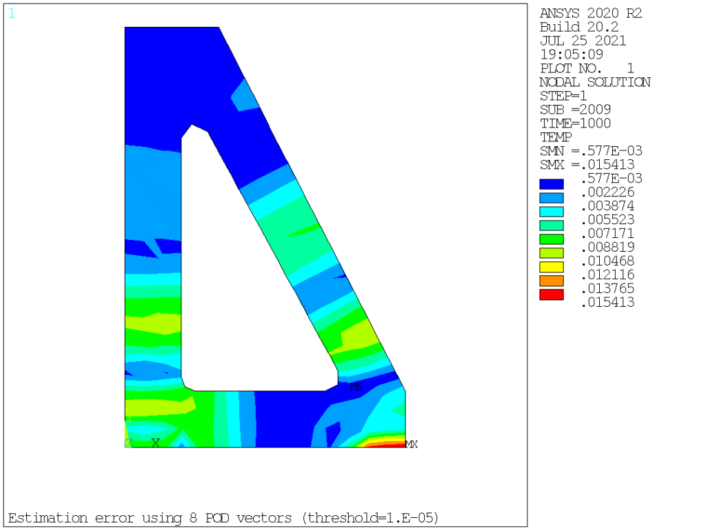
Now, let’s apply POD magic to these values and see what happens. To test the method efficiency, we will assume decreasing values for the threshold parameter, and extract the maximum RMS error in terms of nodal temperature over the entire model.
| Config# | Threshold | Model Order | Max. Nodal Error [K RMS] |
| 1 | 1e-2 | 2 | 1.76 |
| 2 | 1e-3 | 4 | 0.60 |
| 3 | 1e-4 | 6 | 0.057 |
| 4 | 1e-5 | 8 | 0.015 |
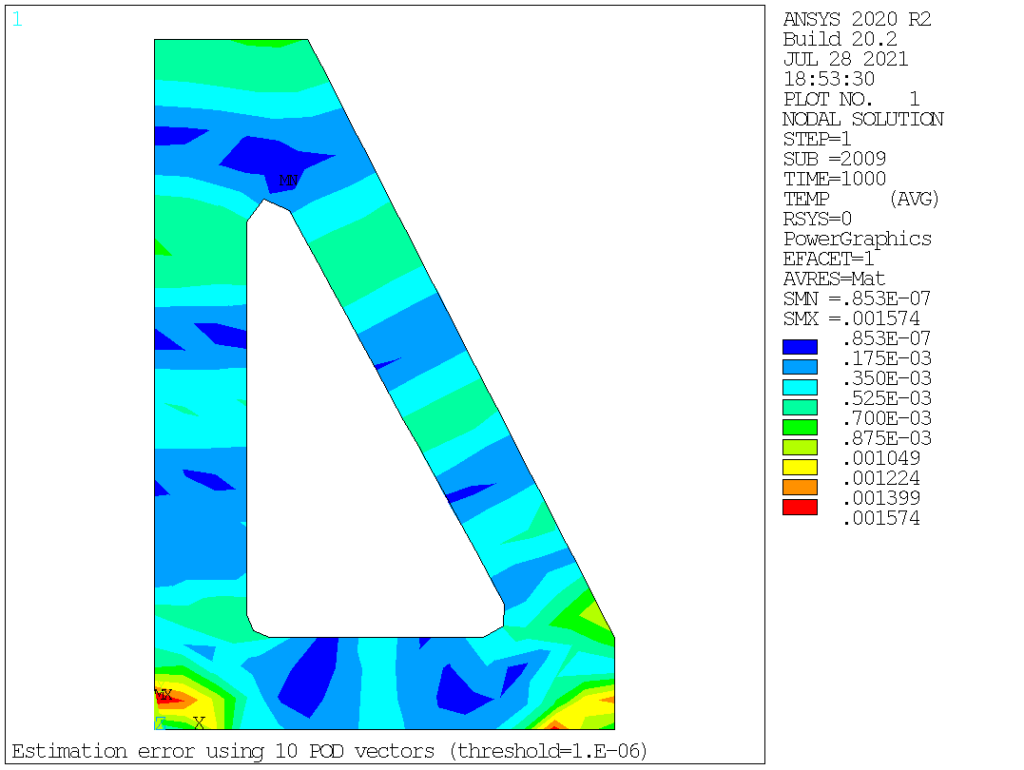
| 5 | 1e-6 | 10 | 0.0016 |
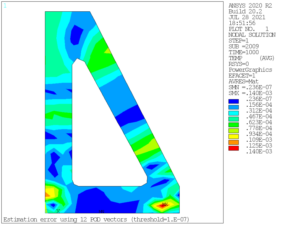
| 6 | 1e-7 | 12 | 0.00014 |
From this, it is quite obvious that the procedure converges extremely rapidly, so that using 8 vectors, one readily reduces the compression error to about 1.5% of the original values, and below 0.01% for 12 vectors, well below the most daring engineering accuracy. It is also interesting to look at the corresponding spatial error distribution, see below. For the first two cases (model order 2 and 4), the maximum error is located about halfway along the heat propagation direction, while for higher order cases, the error is mostly localized at the bottom of the bracket.
Quite impressive, if you ask me. Now, let’s turn on to visually inspecting those POD vectors, which are so efficient at capturing the physics at hand:
POD Vectors unveiled
POD (aka left singular vectors) order 1 to 9 are as follows:
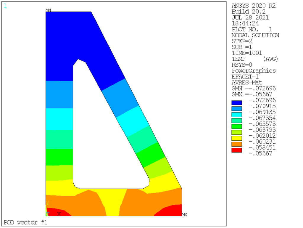


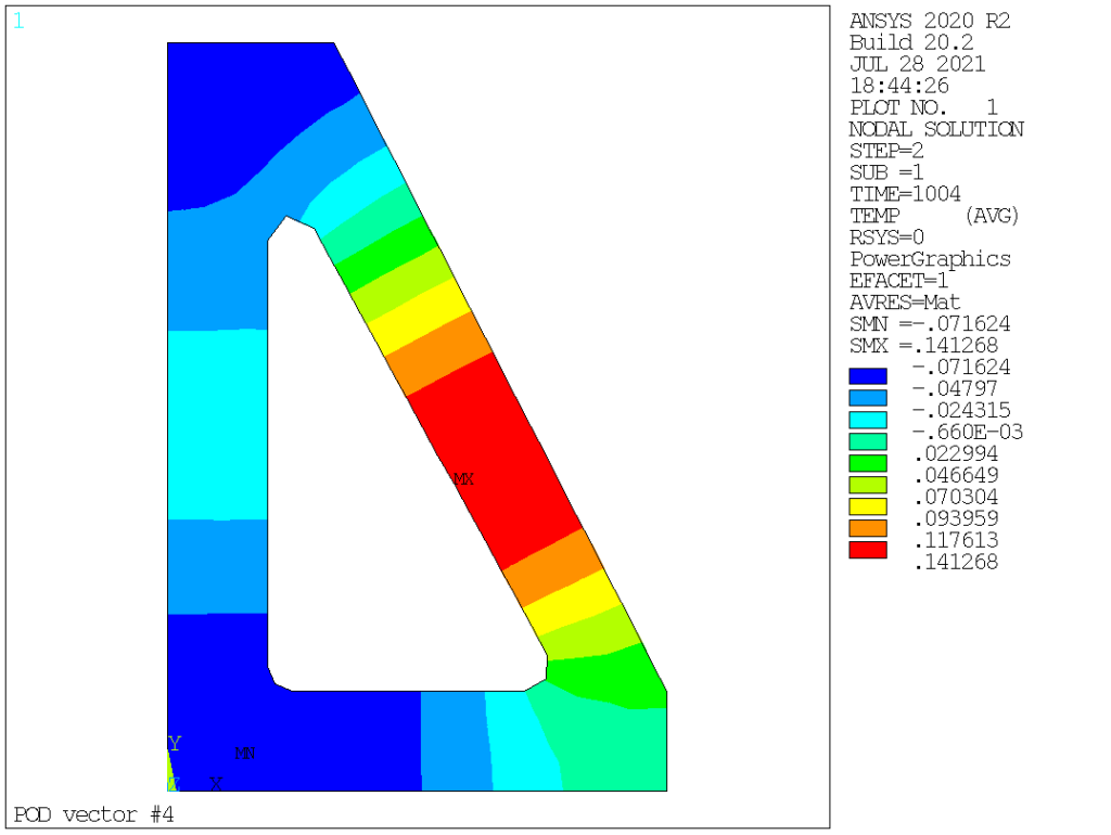
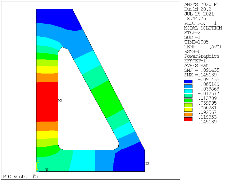
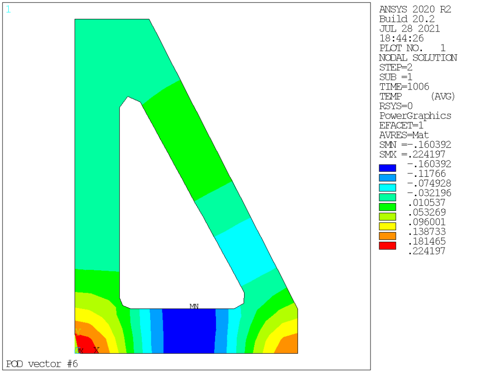
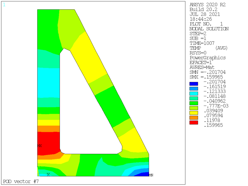
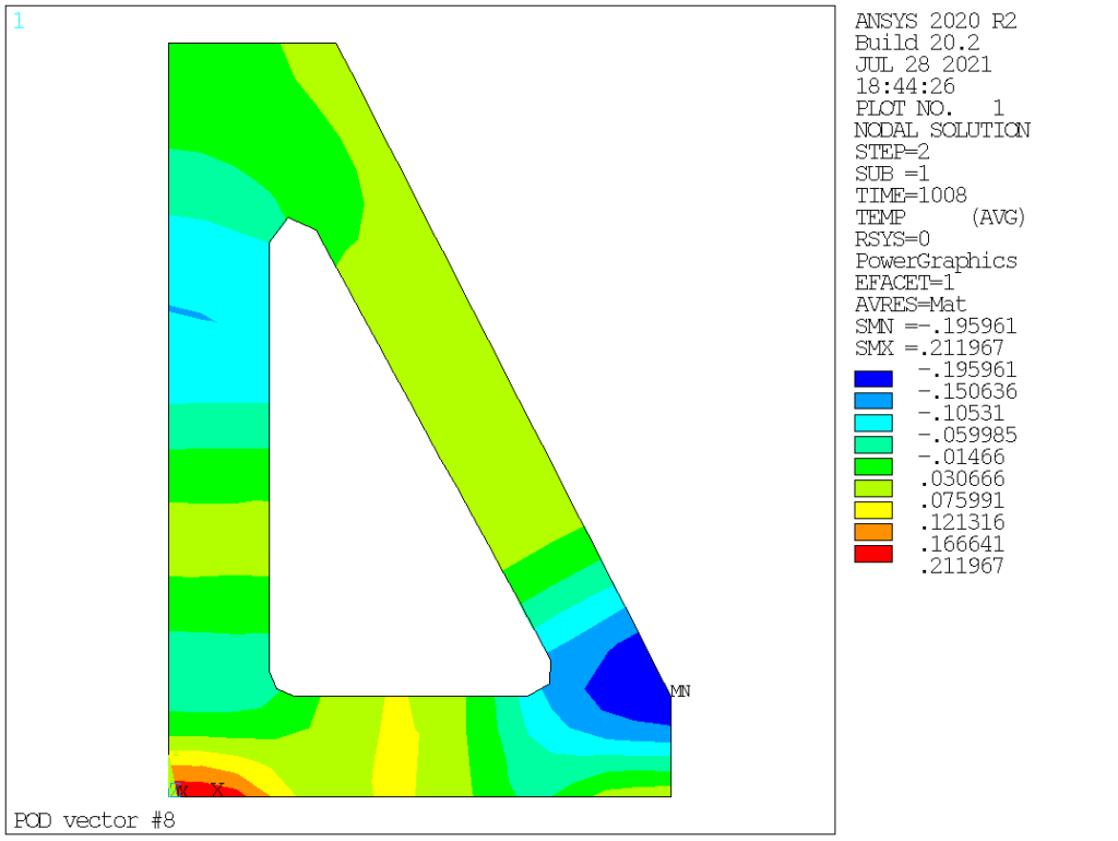
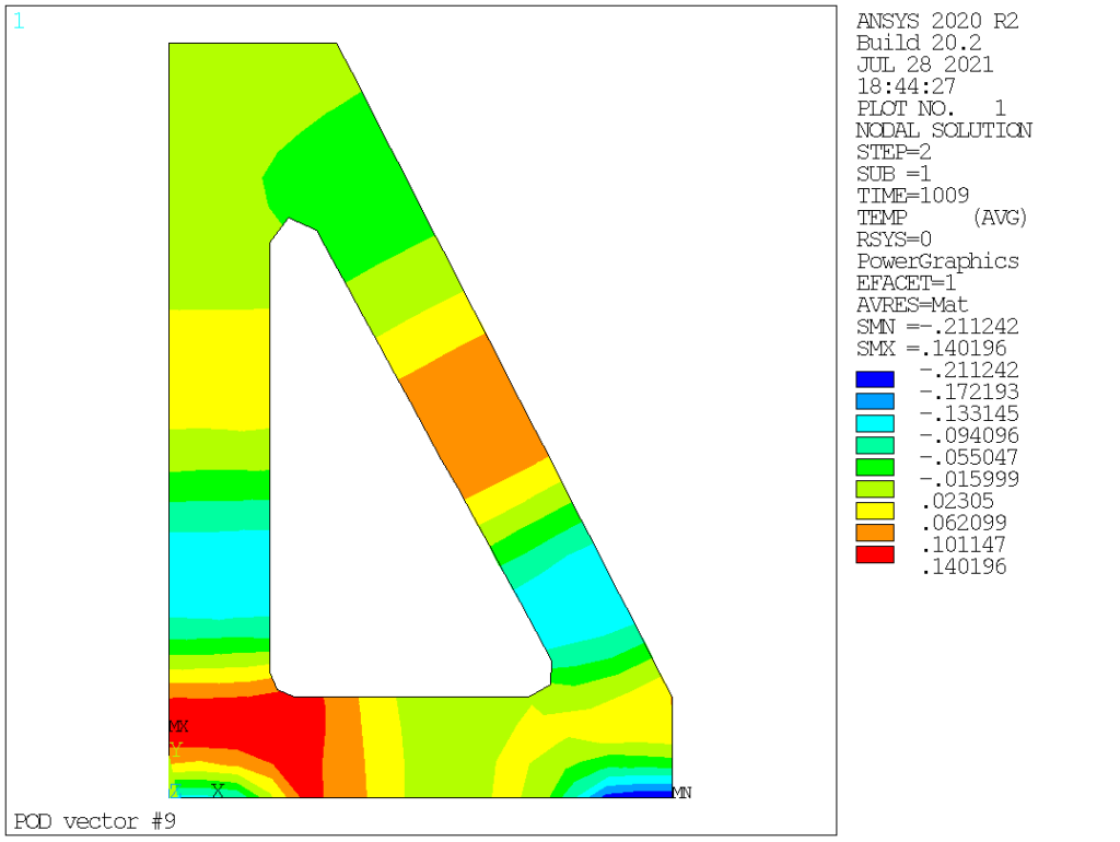
Obviously we see that POD vectors are only loosely connected to normal modes. In this particular case, the mass (thermal inertia) is homogeneous, hence the very first POD and normal modes are somehow similar, but this is not the case for the other modes: POD vectors corresponds to temperature distribution that are actually existing in the solution (based on the specific loading applied, both space and time-wise), ranging them in terms of contribution, while normal modes capture all possible temperature distributions, ranging them from lowest to highest «strain energy» (or, in thermal terms, from the longest to the shortest time constant).
To reiterate, normal modes are orthogonal with respect to the «mass» and «stiffness» matrices (here, thermal capacity and conductivity) while POD vectors are orthogonal with each other. So far, so good. Now, we have a means to compress data, in our case from 228 nodal values per time point down to a mere dozen.
A word of caution about threshold : in ANSYS, this is interpreted as the ratio of the current eigenvalue to the first (largest one). To clarify this, one can inspect the sigma matrix (which is actually a diagonal matrix, and stored as a vector). Dumping this vector to a text file one can readily check that actually, by requiring a threshold of 1e-2, only the first two POD vectors were required. Also, the decreasing rate is really both very fast and very steady, as illustrated by the singular values vector entries (see below). The amplitude decreases by a factor of 10 every other POD vector, down to 1e-12. This is in total contrast with normal modes, especially with thermal problems, for which the convergence rate is generally extremely slow.
SIGMAVEC
- Object : C_VecPi Vector
- Scalar : Double
- Dim : 1000
- In Core : 1
- Values :
 2.060e+04   4.001e+02   3.170e+01   1.377e+01   6.441e+00
 1.593e+00   4.226e-01   1.794e-01   7.203e-02   2.394e-02
 7.098e-03   2.147e-03   6.429e-04   2.468e-04   6.185e-05
 1.837e-05   4.156e-06   8.188e-07   1.779e-07   4.781e-08
 6.798e-09   1.133e-09   2.100e-10   4.304e-11   8.585e-12
 4.392e-12   2.057e-12   1.686e-12   9.462e-13   7.568e-13
 6.757e-13   5.885e-13   4.543e-13   4.237e-13   4.094e-13
 4.044e-13   3.976e-13   3.837e-13   3.814e-13   3.777e-13
 3.709e-13   3.666e-13   3.601e-13   3.575e-13   3.525e-13
 3.483e-13   3.472e-13   3.418e-13   3.386e-13   3.365e-13
 3.355e-13   3.311e-13   3.300e-13   3.254e-13   3.239e-13
 3.223e-13   3.190e-13   3.159e-13   3.124e-13   3.108e-13
  ...
Other tests conducted with thermal conduction/diffusion models in the range of up to 100k DOF showed the exact same trends. It was never necessary to include more than a dozen POD vectors to achieve excellent convergence (relative error below 10^-4). The POD reduction process, by itself, never required more computation time than about one transient time step.
Summary and Conclusion
As we know, engineering simulations generate significant quantities of output data, which are certainly not spatially random -even if the forcing function is- but always organized by the physics of the system. Hence, a compression tool like POD will find repeating patterns (correlation) between DOF responses, and find an optimal base for reduced order representation of system response, capture both system dynamics and forcing function characteristics.POD reduction will always function, on one condition: the data used for identification must be rich enough, which in turns requires the loading to be «harsh» enough. (And yes, engineering judgement will still be around for a while, very much so).
This nice property can be used to our advantage for situations where large data volumes must be stored. But even more important, for all situations where linear downstream analysis are to be subsequently performed, it opens the possibility to directly estimate responses by linearly combining the unitary responses of a handful of base vectors. This can be very handy for say-thermal elastic problems, for which the mechanical analysis can be obtained «for free», once the thermal transient analysis has been performed. The additional cost of projection of the thermal solution onto the POD basis, and the estimation of the mechanical response are numerically inexpensive, and this can be invaluable when long, complex (a-periodic) transients must be analyzed.
Beyond that, for truly non-linear problems, POD method allows to find the lowest dimensional space in which to search for a solution, leading to efficient model reduction techniques.
Both aspects will be treated in upcoming articles so stay tuned.
Happy reduction!
References
- [1] Brunton and Kuntz – Data Driven Science & Engineering : Machine Learning, Dynamical Systems, and Control
- [2] https://gregorygundersen.com/blog/2018/12/10/svd/
- [3] https://ocw.mit.edu/courses/mathematics/18-065-matrix-methods-in-data-analysis-signal-processing-and-machine-learning-spring-2018/video-lectures/lecture-17-rapidly-decreasing-singular-values/