Working Wonders with ADPL Math - Ep 04: Data Reduction Applied To Thermal-Elastic problems - Page 2 of 4

Thermal stress induced by thermal shock in a tee-shaped junction

Let’s apply our nice principle to a typical example that is: a tee-junction. Whenever experiencing sudden temperature change, the inner and outer regions of the pipe will momentarily have different temperature (the diffusion process will limit the through-thickness heat transport), and compressive mechanical stress will develop mostly in the inner region, with a time constant that can easily be estimated by hand. Additionally, in the case of fluid flow being stopped in either the branch or run, each part will also experience different temperatures, and again differential dilatation and mechanical stress will develop, this time at the junction.

The FEM is shown hereafter, comprising 96 000 elements and 116 160 nodes:

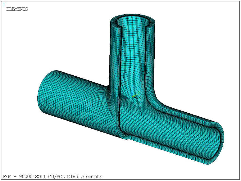
A finite elements model dedicated at capturing the through-thickness bi-metal effect

In this example, we assume a generic, 48×6 tee, made of steel (CTE = 15ppm/K, density of 7.85, thermal conductivity of 15W/m/K, specific thermal capacity of 500J/g/K, elastic modulus of 200 GPa). This gives a thermal diffusivity of 3.8mm²/s, to be compared with the thickness of 6mm. The time required for heat to travel a distance of 6mm can therefore be estimated to be: $t_{diffusion}=\dfrac{6^2}{3.8} \simeq 10s$ .

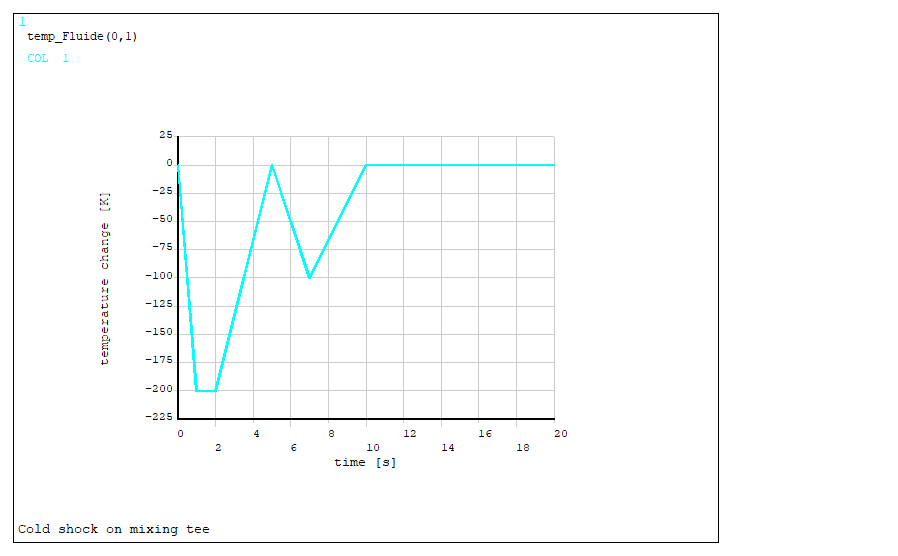
Now, let’s assume a “cold plug” suddenly travels through the run (here: the horizontal part), while the fluid in the branch remains standing. The fluid bulk temperature in the flow would assume a (purposedly) very sharp temperature change:

Linear decrease of 200K between t=0 and t=1s
Plateau for 1s (t=1 to t=2)
Slower, linear return to initial temperature in 3s (t=2 to t=5s)
Second decrease, with half the initial amplitude, and twice the duration (i.e. 50K/s) (t=5 to t=7s)
Return to initial temperature between t=7 and t=10s

The total simulated duration is 100s (but only the first 20s are shown for the sake of clarity).

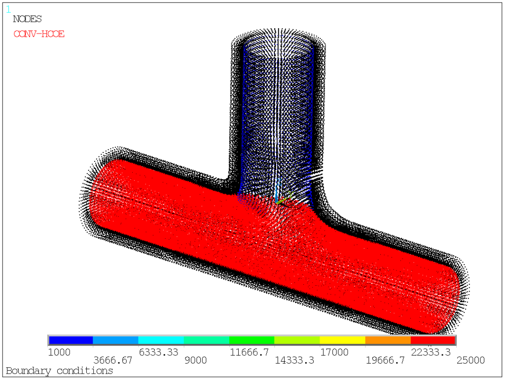
The coefficient of heat exchange in the region of fluid flow will obviously be much higher than in the stagnant region. To obtain a high contrast, we select values for the film coefficient value of 1000 and 25 000W/m²/K, respectively. Elsewhere, we assume negligible heat fluxes (i.e. adiabatic boundaries).

In terms of boundary conditions, we assume that radial dilatation is free, but axial direction is blocked on the upper pipe.

Convection film coefficient distribution (fluid is reamains stagnant in the vertical pipe)

Now, we can put our method to the test of this highly dynamic thermal event. First of all, we let ANSYS solve for the temperature fields. Following the rules of the trade, we select initial time-step size based on thermal diffusivity and element size (here: 0.2mm radially, so initial time step is a bit less than 0.01s), and then let auto-time stepping algorithm do its job. We end up with a set of 157 results, all defined on 116kDOF, so approximately 18 M nodal temperatures values.

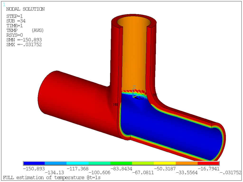
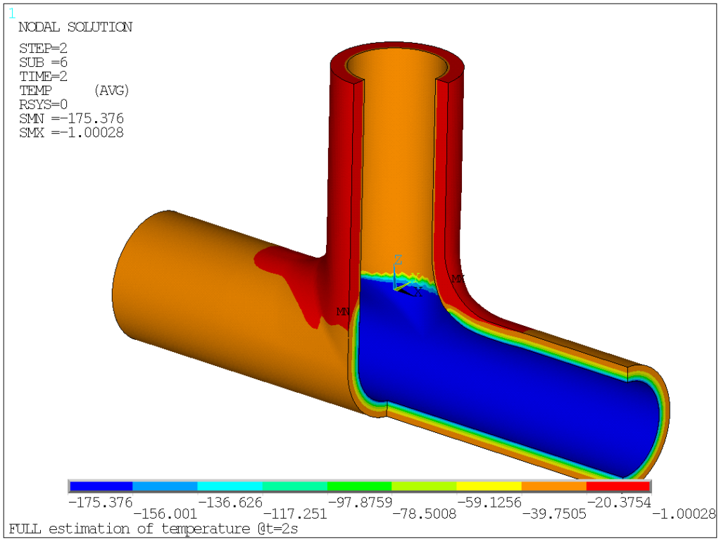
Temperature distribution at a few key points in time are given:

At the end of fluid temperature decrease (i.e. at t=1s)
At the end of the plateau (i.e. at t=2s)

Temperature distribution at the end of temperature jump.

Temperature distribution at the end of temperature plateau

Now, we can apply the SVD procedure to this rather huge volume of data. Let’s import this, using the snapshot matrix into the APDL Math workspace, as a dense matrix, using the command *IMPORT.

*DMAT,X,D,IMPORT,RST,myResultsFileName.RTH,1,nbSnapshots

To this, the code answers nicely:

  Import Data From File RUN_THERMAL_FULL.RTH (Format=RST)

  IMPORT SOLUTION : Nodal Solution
  DATA SETS       : [1,157]

Well, I don’t know about you, but reading this rather large file on a small machine (16Gb intel i3) only requires 0.14s. OK, that’s not real processing power but mere I/O, however this step alone could have been excruciatingly slow, completely ruining the total process efficiency. As it shows, it doesn’t!

Going one step further, we can now do the actual compression. We specify a tolerance of 0.001, to be compared with the defaults (see previous post for explanations).

Allocate a [157][157] Dense Matrix : VCONJ
 (TOLERANCE = 0.001)
                MATRIX SIZE AFTER COMPRESSION : 7

And this is where the beauty of this appears. Firstly, the POD basis only includes 7 vectors, instead of 157, so that the time required for structural analysis can be decreased by a factor of about 20. And, secondly, the required CPU for SVD reduction is 1.73s. I don’t know about you, but I have had difficulty believing this, so I repeated the operation with various settings, and of course the results change (I/O can play a role) but the basics are demonstrated: SVD reduction is numerically both very fast and efficient. As a side note, performing the same operation with Matlab requires about 4.1s.

As a matter of fact, I did a sensitivity study to check the convergence rate, as shown in the table below:

Trial	Threshold [-]	CPU [s]	POD vectors	Error L2 / LINF
1	10^-1	2.3	2	1.3 10⁴	1.2 10³
2	10^-2	2.2	4	1.5 10³	3.7 10²
3	10^-3	2.4	7	1.3 10²	2.2 10¹
4	10^-4	2.3	11	7.4 10⁰	1.6 10⁰

The nothing-less-than-astounding convergence rate of SVD applied to thermal shock

As expected the reconstruction error decreases with a rate similar to the threshold value. Surprisingly, the reconstruction error (estimated using the *NRM function, applied to the reconstruction error matrix) gives L2 values that are larger than the L_inf norm. The documentation is not really helpful in order to understand this behavior.

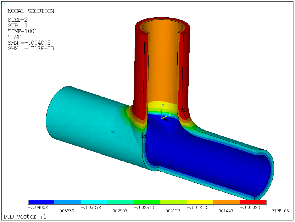
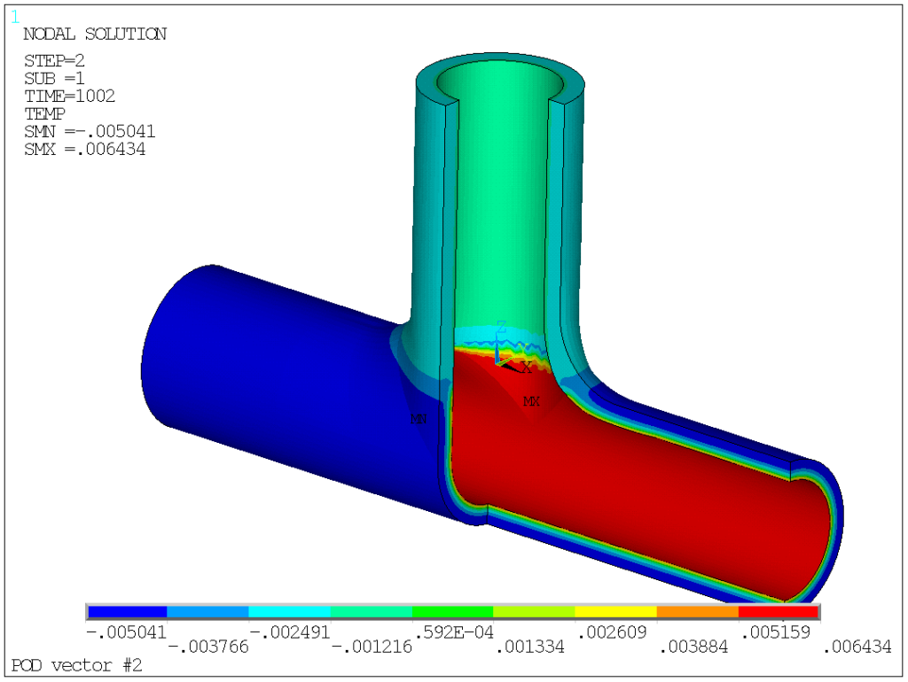
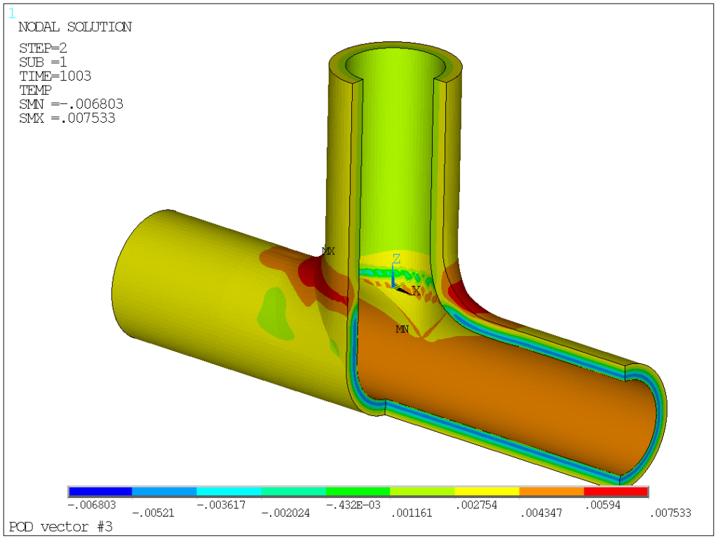
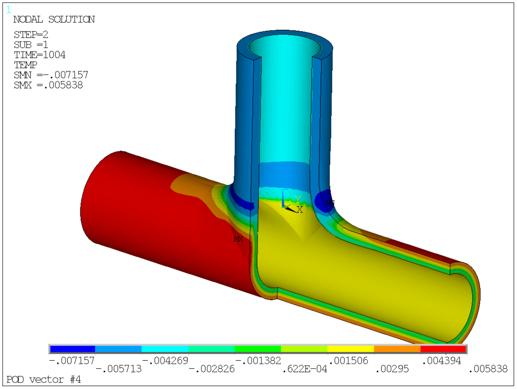
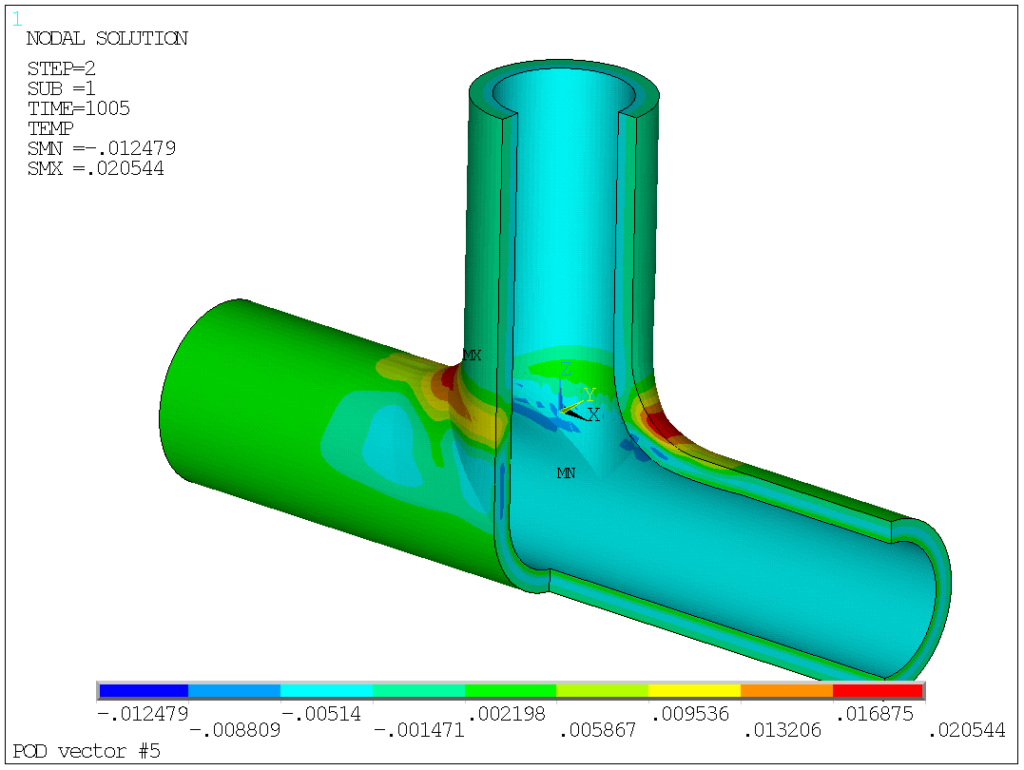
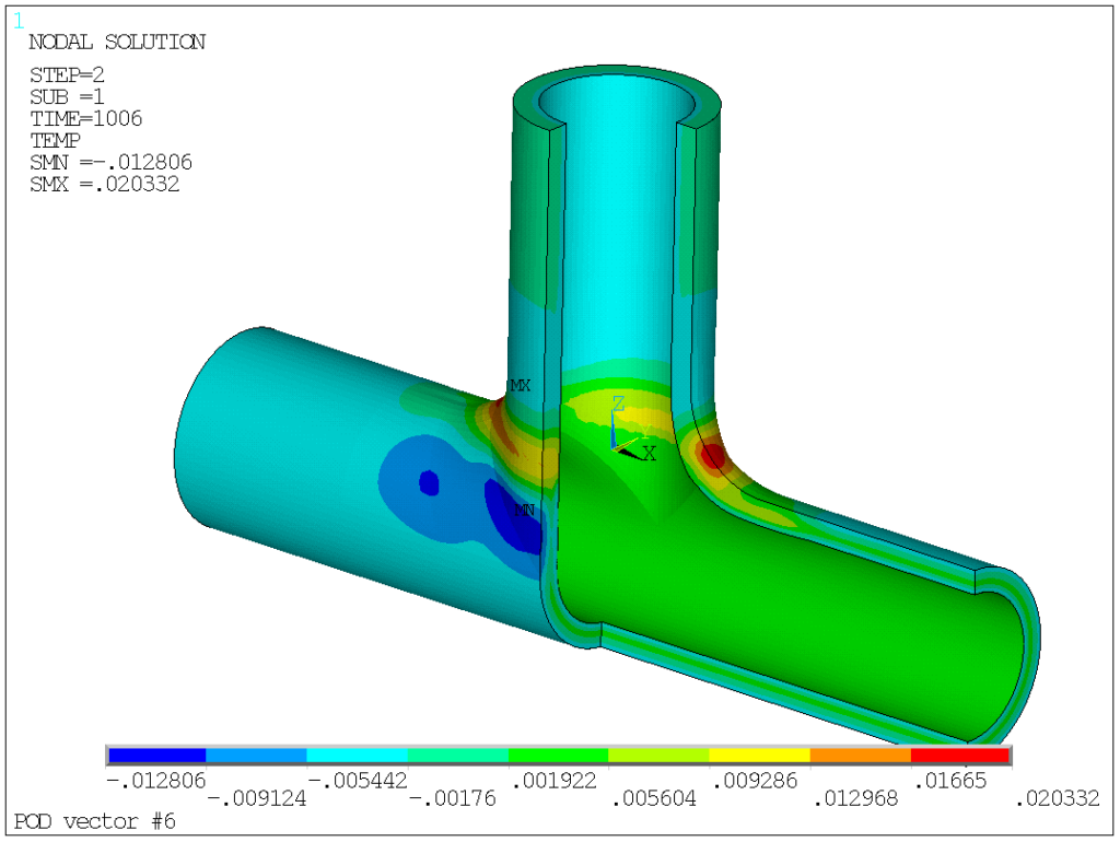
For the time being, I assume that a threshold of 10^-3 is largely acceptable for engineering purpose. What do these magnificents 7 POD vectors, worth 157 ordinary results look like? Here are they (I removed one quadrant for better readability, since obviously, the results are symmetric with respect to the X=0 and Y=0 plans).

POD vectors 1 in-phase temperature change in branch and run, while vector 2 and 3 capture the through-thickness temperature gradients. Vector 4 corresponds to heat exchange between branch and run (out-of-phase temperature variations). Modes 5,6, and 7 are all local modes at the junction.

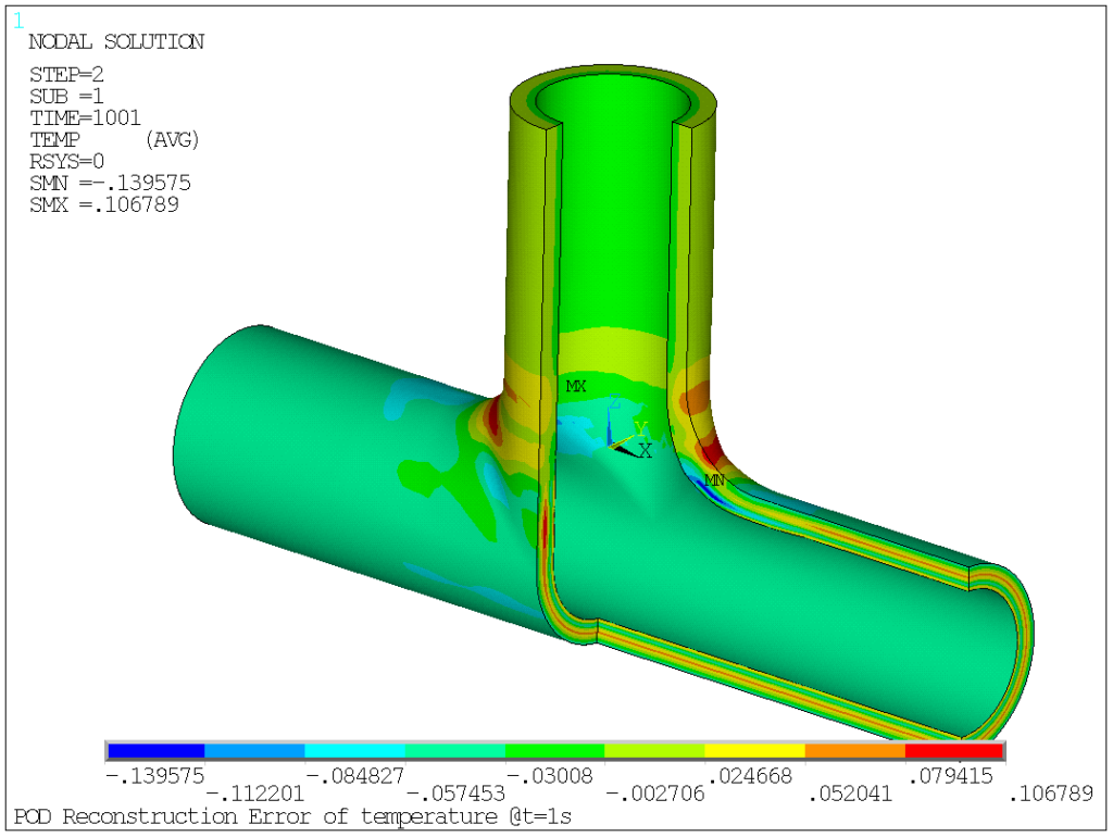
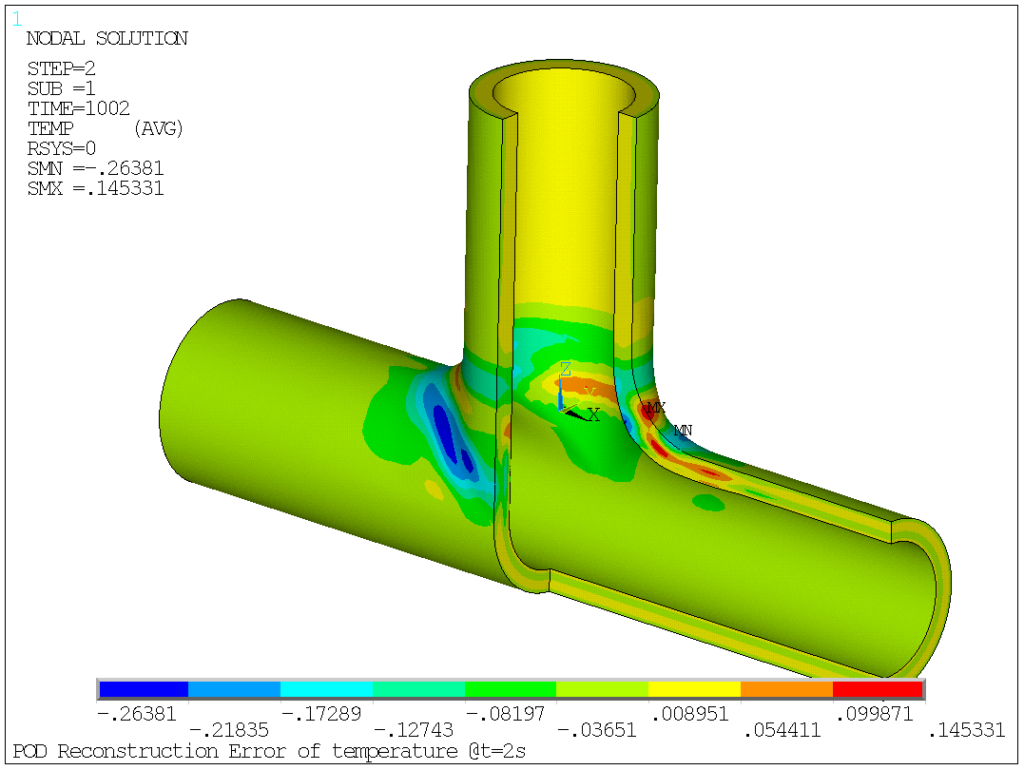
Now, we can also estimate the reconstruction error induced by the POD method. Here, using a threshold value of 10^-3 (i.e. 7 POD vectors), the error has been mapped on the structure at t=1 and 2s, to get an estimate of the error amplitude and localization. Clearly, the reconstruction error is really small (of the order of 10^-1K, to be compared with a temperature jump of the order of 2.10²K), so a relative error of less than 10^-3

Reconstruction error of temperature distribution at the end of temperature jump.

Reconstruction error of temperature distribution at the end of temperature plateau.