Working Wonders with Dynamic Instrumentation – Ep02: Instrumental Noise Identification

Practical Method, Limitations and Results

As we know, the above formula is only valid in a mathematical -i.e. idealized- sense. Actual values will be statistical estimated of the 4 required quantities (And all of them will only converge to their final value after a number of averages which may or may not be achievable in practice). Again, we refer to [1] for details, but for now let’s just remind that the relative error on obtained using n averages (i.e. averaging n short term DFT’s) can be approximated as:

(1)  

Now, let’s say that the noise PSD we are looking for accounts for 50 % of the total PSD (this, of course, we don’t know beforehand. I am just making things up to clarify the discussion). And, in order to be in a position to compare various sensors and setups we wish for no more than 10 % uncertainty on the instrumental noise estimation .

It follows that we should be able to estimate PSD down to 5 % relative error, so that a minium of 1/(0.05)^2= 400 averages is required. That’s already a lot of data to be collected, we will come back to this point in an upcoming article.

Now let’s make a numerical test case. We will assume 3 signals recorded for a duration of 1000s, originating from different sensors.

Let’s say our 3 sensors have noise standard deviations within ± 20 %, and sensitivities within 5 %.

A short Matlab/Octave script can be written for that purpose. Let’s select the numerical parameters. We select comparable amplitudes (1-sigma deviation) for both the mesurand (i.e. actual physical quantity existing at the sensors input) and the instrumental noise.

fSampling=256;  % sps   - sampling frequency
duration=1000;  % s     - simulated record duration
 
% assumed RMS amplitude for signal (i.e. mesurand)
sigmaX=1e-4;
 
% assumed RMS amplitude for white noise (1-standard deviation)
sigmaN1=0.8e-4;
sigmaN2=1.2e-4;
sigmaN3=1.0e-4;

First, we create our test signals :

%% create mesurand and noises realization
nSamples=fSampling*duration;
 
signal=sigmaX*randn(nSamples,1);
 
n1=sigmaN1*randn(nSamples,1);
n2=sigmaN2*randn(nSamples,1);
n3=sigmaN3*randn(nSamples,1);
 
% superimpose signal and noise to get measured quantities
% This is what we can observe in real life.
y1=signal+n1;
y2=signal+n2;
y3=signal+n3;
 
% merge 3 signal vectors into a signal matrix (nSamplesx3). 
y=cat(2,y1,y2,y3);

Now, let’s compute the observed signals cross-power spectral density matrix. Using the ‘MIMO’ option, the result is stored as a 3D matrix, with size (nFFTlinesxnChannelsxnChannels) :

%% Extract noise from redudant measurements

% Step1: Create Cross-PSD matrice
nFFT=fSampling;         % 1Hz frequency resolution
nOverlap=nFFT/2;
nAverage=nSamples/nFFT;
window=hanning(nFFT);   % window
df=fSampling/nFFT;      % frequency resolution  
[Pyy,f]=cpsd(y,y,window,nOverlap,nFFT,fSampling,'mimo');

Lastly, let’s estimate the extraneous noise for each of the 3 channels:

%  Step2: Extract various noise PSD's
N11=extractExtraneousNoise(Pyy,1,2,3);
N22=extractExtraneousNoise(Pyy,2,3,1);
N33=extractExtraneousNoise(Pyy,3,1,2);

The local function extractExtraneousNoise function simply reads :

function Nii=extractExtraneousNoise(Pyy,i,j,k)
    Pii=Pyy(:,i,i);
    Pji=Pyy(:,j,i);
    Pik=Pyy(:,i,k);
    Pjk=Pyy(:,j,k);
    Nii=Pii-Pji.*(Pik./Pjk);
end

Now, how good are the results? I let you decide.

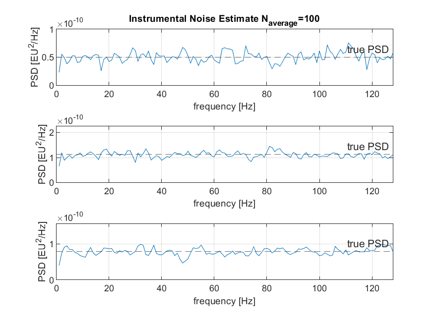
A few comments follow :

-the PSDs are not quite smooth, but this was to be expected : using 100 averages, the spectral estimator has a standard deviation of 10 %, so that we have to expect individual results to be contained in +/-30 % around the « true » value.

-the total variance is perfectly well estimated, the deviation to the true value being less than 1 %, whichever the channel. This is also to be expected (the deviation of the total energy being equal to the deviation of the individual components divided by the number of terms in the sum, here there are 128 of them since the analysis bandwidth is 128Hz and we have selected a 1Hz frequency resolution). Hence, the 1-sigma relative uncertainty is 0.1/(128)^(1/2)~0.004, i.e. a 3-sigma relative error of about 2.4 %.

So far, so good, now let’s turn to a real life test case.