Categories
Technical Literature

Working wonders with dynamic instruments – Ep 01: Resolution limits

This post comes as an answer to the question I perhaps heard most often when troubleshooting optomechanical devices. When faced with a anything other than an optical sensing device (i.e., an inertial sensor), the optomechanical specialist immediately (and rightfully) wonders:

What is this sensor’s (instrument, setup) resolution?

As it is, this is the perfect example of a question that takes 5 words to ask but requires a relatively lengthy discussion to answer (except for the obvious “it depends” which indeed is only optimal in terms of conciseness). Reading what follows will hopefully provide a satisfying answer for anyone interested in the question.

Inertial Sensors

There are many virtues that make inertia sensors (either velocimeter or accelerometers) attractive. To name only a few, they are compact, relatively economical, have excellent linearity. Importantly, since they are inertia based, they do not require any external reference, making it possible to know exactly which part is moving, because they are delivering a signal corresponding tochanges in position of the attached object (contrary to optical based, or capacitive based sensors etc which deliver a signal correlated to changes in separation length between two objects). Also, they can provide quantities along any direction, and come into a variety of flavor, that is, with or without integrated electronics, the latter being fit for survival in harsh environments, possibly enduring years of operation with high-energy photons exposure.

Now, an immediate question is, how to convert information produced as velocities or acceleration into lengths? There would be integration (single or double) involved, which inevitably poses important limitations:

  • Only changes in position are detected, and since the reference (initial value) of position is unknown, so obviously only variation about a time-averaged position can be produced.
  • Because of first principles, DC (i.e. constant) components cannot be measured (nor do they need to, unless one wishes to double-check local gravity). The lower limit is dictated by the coil/spring natural frequency (in the case of a velocimeter) or by the crystal leak resistance (in case of a piezoelectric accelerometer).
  • Integration involves accumulating signals, but so does errors: hence integrating ‘forever’, i.e. without any high-pass filter, will result in erroneous drifts that will soon render the integrated signals indecipherable. We will come back to this point in a minute.

Resolution and Usable Bandwidth

Now, letting aside for the moment the discussion about the sensor’s usable bandwidth, we need to recognize that inertial sensors have no “threshold” effect, hence their effective resolution will be dictated by their intrinsic noise only. An excellent discussion is made in [1], which I will not repeat here.

For the moment, it suffices to say that noise is by definition a wide-band process, hence before trying to quantify a noise amplitude, one should start by specifying the bandwidth that is of relevance for the problem at hand. Starting with the most simple situation, that is the “white noise of the engineer”, the instrumental noise variance simply scales linearly with the bandwidth:

{\sigma} ^ {2} = \int_{f_1}^{f_2} {\Phi_{nn}(f ) df \simeq {\Phi_{nn} \times (f_2-f_1)

with:

\PhiΦ_{nn}(f): Power Spectral Density [unit EU^2/Hz]

The approximation assumes small variation of PSD about its mean value (i.e. a “flat” spectrum).

Inertial sensors, have most of their bandwith dominated by thermal noise (i.e. uniform power spectral density), this means a single value is enough to characterize the instrument noise. This, however, is not exactly true at the lower end (where flicker noise dominates, see [2]).

In practice, the RMS amplitude velocity (or acceleration) noise would scale as the bandwidth, and will be independent of the starting or ending frequencies.

Now, this is not the case anymore if a single integration is needed. Namely, for a single integration the variance would read:

{\sigma_{single integration}} ^ {2} = \int_{f_1}^{f_2} \dfrac{\Phi_{nn}(f )}{4 \pi^2 f^2} df \simeq { \dfrac{\Phi_{nn}}{4 \pi^2} \times (\dfrac{1}{f_1}-\dfrac{1}{f_2})

Completely opposite to the case without integration, the variance is dominated by the low frequency content. In practical terms, there are orders of magnitude separating lowermost and uppermost frequencies so that only the former is of relevance, and the previous expression can be simplified into

{\sigma_{single integration}} ^ {2} \simeq \dfrac{\Phi_{nn}}{4 \pi^2 f_1}

This is even more pronounced when one needs to apply a double integration, in which case the variance due to instrumental noise reads:

{\sigma_{double integration}} ^ {2} = \int_{f_1}^{f_2} \dfrac{\Phi_{nn}(f )}{16 \pi^4 f^4} df \simeq { \dfrac{\Phi_{nn}}{48 \pi^4} \times (\dfrac{1}{f_1^3}-\dfrac{1}{f_2^3})

where the approximation again only holds if the noise spectrum is flat. By an argument similar to the previous one, this expression can further degenerate into:

{\sigma_{double integration}} ^ {2} \simeq { \dfrac{\Phi_{nn}}{48 \pi^4 f_1^3}

Now, clearly, we have a very strong dependency of intrinsic noise on the selected bandwidth, or more accurately on the lower end of the bandwidth. Dividing the lowermost frequency by a factor of 2 will increase the intrinsic noise by at least a factor of 8 (and in practice, a bit more than that as soon as flicker noise comes in).

Categories
Technical Literature

High stability systems: V-shaped optical reference cavity

Our article, dealing with a system developped at the LSCE by Mathieu Casado and Samir Kassi, has been published in Applied Physics B journal.

You can find it here:

https://rdcu.be/cHSOj

It is a companion paper to a previous article (Part 1) that puts emphasis on the actual performance achieved by the system.

This study, orignal started in the year 2017, was the reason why we developped thermal modal analysis/thermal-mechanical harmonic capabilities. Without them, we were at a loss when trying to decide wether our design was still lacking stability, and what should/could be removed or added to have a design that is correctly balanced.

As a supplementary material, we have added the principles and formulas outlining the procedures, in the hope that it can be of use to the general opto-mechanics community.

Categories
Technical Literature

Working Wonders with ADPL Math – Ep 04: Data Reduction Applied To Thermal-Elastic problems

Data reduction for real-world applications

In the previous post of this series (here: Working Wonders with ADPL Math – Ep 03: Data Reduction Fundamentals), we have seen that using a bunch of APDL Math commands, it is possible to reduce large volume of data (i.e. snaphots) very efficiently. Now, data reduction method like POD is obviously attractive but reducing results file size is rarely a major concern. More often than not, obtaining simulation results with minimal computational effort is what we are looking for.

So, how can we use POD for practical situations? There are a bunch of possibilities, that we will explore in the upcoming episode of this series. Here, we will begin with the simplest and straightforward situation one could think of: thermal elastic simulations.

Thermal-elastic simulations from data reduction perspective

There are many instances where one needs to efficiently execute thermal-elastic situations. From a fatigue point of view, for example, it is useful to run analyses with numerous realistic transients (possibly using actual records) rather than a single, penalizing transient, with generally huge, but unknown built-in safety margins.

In such a situation, one will generally solve the problem sequentially:

  • First thermally, in the time-domain, possibly accounting for non-linear phenomena and/or time-dependent characteristics. Here, the emphasis needs to be put on capturing temperature elevation as well as gradients which are drivers of flexural stresses.
  • The resulting temperature snapshots are then feed into a structural model, where inertia effect are neglected. Hence, static structural solutions are needed.

To emphasize, capturing the exact temperature or stress time-histories is not mandatory: the figure of merit here will be stress range, i.e. extreme values.

Now, the regular approach would be to solve in the time domain for the temperature distribution in the structure T(x,t) at a series of instants t1..tn. From this, a series of n structural solutions would be performed, producing the structural displacement U(x,t), and derived quantities such as stress/strain. Note that, the structural displacements could be estimated “on the fly”, as structural displacement at time “t” obviously doesn’t depend on past or future values.

Alternatively, the POD approach would consist in:

  1. Evaluating the temperature distributions at all time points, i.e. the snapshot matrix (n_{DOF}\times n_{instants}).
  2. Compressing those snapshots using SVD method: this produces a set of nodal amplitudes (n_{DOF}\times n_{POD}) and POD vectors amplitudes(n_{POD}\times n_{instants})
  3. Evaluate the individual structural response for each of the thermal POD vectors .
  4. Combine the individual structural responses to obtain the physical response at all locations and time points.

The expected computational gain is clearly related to the ratio between the number of time points and that of the required POD vectors, and we should expect the solution time reduction to be close to that value (keeping in mind that the SVD decomposition by itself will only require an additional solution time comparable to one additional time point).

Categories
Technical Literature

Working Wonders with ADPL Math – Ep 03: Data Reduction Fundamentals

What are we doing here?

This post may come as a surprise to many, as ANSYS APDL is at its core a tool aiming at simulating physical phenomena so that «data reduction», being more oriented to the data analysis community, might sound a bit out-of-place.

As a matter of fact, being a numerical tool, it does have ubiquitous applications and -as we shall shortly see- it can be also beneficial to down-to-earth, goal-oriented folks like say -engineers.

Browsing the APDL Math commands, I started being curious about the *COMPRESS command, which I had so far ignored: as it was, I had assumed that it merely was a functionality aimed at compressing sparse matrices, i.e. a lossless procedure, detecting and eliminating near-zero entries. And yes, that’s exactly what it can do, but there is more to it: it will also compress data using Singular Values Decomposition (SVD), which is probably one of the most important numerical tool there is. This is not the place to provide too much background on the topic, and for those interested there is a wealth of books and articles on the subject, one prominent contribution being the online videos by Steven Brunton and Nathan Kuntz, see [1] for an introduction.

Before discussing applications, I will briefly introduce the topic of SVD, how it relates to data compression, and which APDL Math capabilities we need to use.

Categories
Technical Literature

Working wonders with APDL Math – Ep 02 : Thermal Harmonic Analysis

Where do we want to go from here?

In a previous post, I tried (and from the feedback I got, somehow succeeded) to introduce the beauty of developing extensions to the core capabilities of ANSYS by means of APDL Math commands.

Now, that was merely an introduction, using but the most simple physics (linear thermal model) and solver (modal thermal). There is of course much more to be expected from such general capabilities as matrix manipulation, and since they are meant to address some “unconventional” needs, it would hardly make sense to go on and try finding the additional capability “everybody was waiting for”.

Hence, I am going to follow the track I started so far, and resume my journey into the wonders of APDL Math with the natural extension of modal analysis that is, harmonic analysis. This might be directly useful to a few readers, and hopefully will be an incentive for users to use the existing solvers for answering their own needs.

Thermal Harmonic Analysis at a Glance

Thermal harmonic analysis is so scarcely used that, as of May 2018, even Google had not heard about it. No, seriously, not a single match. Gulp. But don’t panic, it is nothing esoteric, really. The concept was introduced as early as the 1960’s (see ref [1]), and is used under one form or the other every time it is necessary to design a system with high immunity against thermal disturbances. Actually, you would encounter it under one form or the other whenever stringent dimensional stability – hence thermal stability – is required.

Specifically, it can provide quantitative answers to crucial design questions:

  • Q: What will be the net fraction of external temperature fluctuations that will propagate into my system?
  • A: Compute Thermal Transmissibility Tr(f) between the “noisy” and the “quiet” side. Once obtained, the temperature fluctuations Power Spectral Density (PSD) on the quiet side will be given by the usual relationship for linear systems (i.e. PSD_{T_{quiet}}=\vert Tr(f) \vert^2PSD_{T_{noisy}}). From this, estimating the RMS temperature fluctuation on the quiet side is straightforward. Even more importantly, it also grants knowledge to the temperature drift rate and its Allan Variance, that in turn allows one to estimate the maximum allowable duration for an experiment .
  • Q: Assuming stability demands are not fulfilled with a passive design: Can I develop an “open loop” frequency response, so as to decide where to put sensors and actuators (heaters) for an active thermal control system?
  • A: Thermal Harmonic response will provide just what you need, that is, the complex frequency response, giving access to gain and phase. This in turn can be used at the system level to decide on the most appropriate sensors / actuators / controller logic configuration
  • Q: Assuming I am working with a purely optical system, how deleterious will short duration fluctuations of light beam?
  • A: Compute the thermal harmonic response of the system at the beam oscillation frequency (or frequencies). The thermal solution can then be used to estimate the severity of thermally induced distortions (either variation of the material’s refractive index with temperature or thermoelastic expansion) on the final optical performance.
  • Q: Assuming I am working with a structural part submitted to complex thermal loading (i.e. randomly distributed, time and space wise), how can I estimate thermal fatigue?
  • A: Thermal fatigue effects can be effectively captured, since Thermal Harmonic Analysis gives access to (complex) structural temperature fields, with no restriction on the analysis bandwidth. These temperature fields can be used to estimate mechanical stress response patterns, just like the ones produced by a conventional random vibration analysis.

Especially when both thermal and mechanical effects are involved, efficiency is of paramount importance, because of two technical hurdles acting in conjunction: Firstly, since mechanical stress is the final quantity of interest, spatial resolution (mesh size) becomes non-negotiable. And secondly, the loading itself spans orders of magnitudes in correlation length and frequencies, hence the model cannot be strictly restricted to the area of interest without introducing severe bias in the results. Running long transient analyses of a finely meshed model with small time steps is exactly what one should avoid doing.

Even if your application does not involve thermal mechanical phenomena, as soon as linear behavior can be granted, you might want to consider harmonic analysis. Working in the frequency domain not only allows for improved insight but it also drastically reduces the computational burden.

Categories
Technical Literature

Working wonders with APDL Math – Ep 01 : Thermal Modal Analysis

As Times Goes By

Do you remember the moment you first heard about ANSYS introducing APDL Math?

I, for one, do, and I have a vivid memory of thinking “Wow, that can be a powerful tool, I’m dead sure it won’t be long before an opportunity arises and I’ll start developing pretty useful procedures and tools”. Well, that was half a decade ago, and to my great shame, nothing quite like that has happened so far. Reasons for this are obvious and probably the same for most of us:  lack of time and energy to learn yet another set of commands, fear of the ever present risk of developing procedures that are eventually rejected as nonstandard use of the software and therefore error-prone (those of you working under quality assurance, raise your hand!), anxiety of working directly under the hood on real projects with little means to double check your results, to name a few.

That said, finally an opportunity presented itself, and before I knew it, I was up and running with APDL Math. The objective of this article is to showcase some simple yet insightful applications and hopefully remove the prevention one can have regarding using these additional capabilities.

For the sake of demonstration, I will begin with a somewhat uncommon analysis tool that should nevertheless ring a bell for most of you, that is: modal analysis (and yes, the pun is intended). You may wonder what is the purpose of using APDL Math to perform a task that is a standard ANSYS capability since say revision 2.0, 40 years ago? But wait, did I mention that by modal analysis, I mean thermal modal Analysis?

Thermal Modal Analysis at a Glance

Although scarcely used, thermal modal analysis is both an analysis and a design validation tool, mostly used in the field of precision engineering and or optomechanics. Specifically, it can serve a number of purposes such as in the following Q&A:

Q: Will my system settle fast enough to fulfill design requirements?

A: Compute the system Thermal Time Constants

Q: Where should I place sensors to get information rich / robust measurements?

A: Compute Thermal modes and place your sensors away from large thermal gradients

Q: Can I develop a reduced model to solve large transient thermal mechanical problems?

A: Working on a modal basis rather than with the full problem allows for the construction of such reduced model effectively converting a high-order coupled system to a low order, uncoupled set of equations.

Q: How to develop a reduced order state-space matrices representation of my thermal system (equivalent to SPMWRITE command)?

A: Modal analysis provides every result needed to build those matrices directly within ANSYS.

Although you might only be vaguely familiar with many or all of those topics, the idea behind this article is really to show that APDL Math does exactly what you need it to do: allow the user to efficiently address specific needs, with a minimal amount of additional work. Minimal? Let’s see what it looks like in reality, and you will soon enough be in a position to make your own opinion on the matter.

 Thermal Modal Analysis using APDL Math

To begin with, it is worth underlining the similarities and differences between structural (vibration) modes and thermal modes. Mathematically, both look very much the same, i.e. modes are solutions of the dynamics equation in the absence of forcing (external) term:

DomainEquation solvedTerms Explained
Structural ([K]-\lambda [M]) \Phi=0[K] = {stiffness \quad matrix}
[M]= {mass \quad matrix}
Thermal([K]-\lambda [C]) \Phi=0 [K] = {conductivity \quad matrix}
[C] = {capacitance \quad matrix}

Now, the fundamental difference is that the eigenvalues have completely different physical interpretations:

  • in the structural case, \lambda= \omega^2, i.e. the eigenvalue is the square of the modal circular frequency
  • in the thermal case, \lambda=1/\tau, i.e. the eigenvalue is the inverse of the modal time constant

This is a direct consequence of the fact that dynamical systems are 2nd order systems, whereas thermal systems are 1st order systems. While after being disturbed the former will oscillate around its equilibrium position, the latter will return to its initial state via exponential decay. Mind you, there is no such thing as thermal resonances!

No big deal, right? Hence, the APDL Math code for Thermal Modal Analysis should be a straightforward adaption of the original. As it turns out, the modifications are quite small. Below is a table comparing input codes to perform both type of analyses, using APDL Math.

StructuralThermal
! Setup Model

 
! Make ONE dummy transient solve to write stiffness and mass matrices to .FULL file
/SOLU
ANTYPE,TRANSIENT
TIME,1
WRFULL,1
SOLVE


! Get Stiffness and Mass
*SMAT,MatK,D,IMPORT,FULL,,STIFF
*SMAT,MatM,D,IMPORT,FULL,,MASS


! Eigenvalue Extraction
Antype,MODAL
modopt,Lanb,NRM,0,Fmax
*EIGEN,MatK,MatM,,EiV,MatPhi
 
! No need to convert eigenvalues to frequencies, ANSYS does it automatically


! Done !

! Setup Model


! Make TWO dummy transient solve to separately write conductivity and capacitances matrices to .FULL file
/SOLU
ANTYPE,TRANSIENT
TIME,1
NSUB,1,1,1
TINTP,,,,1
WRFULL,1


! Zero out capacitance terms

SOLVE
! Get Conductivity Matrice
*SMAT,MatK,D,IMPORT,FULL, Jobname.full,STIFF
! Restore capacitance and zero out conductivity terms

SOLVE
! Get Capacitance Matrice
*SMAT,MatC,D,IMPORT,FULL,,STIFF
 
! Eigenvalue Extraction
Antype,MODAL
modopt,Lanb,NRM,,0,1/(2*PI*SQRT(Tmin))
*EIGEN,MatK,MatC,,EiV,MatPhi
 
! Convert Eigenvalues for Frequency to Thermal time Constants
*do,i,1,EiV_rowDim
Eiv(i)=1/(2*PI*Eiv(i))**2
*enddo
 
! Done !
 
APDL/APDLMath for structural and thermal modal analysis

The only data requested from the users is the number of requested modes (NRM) as well as the upper frequency (or for that matter, the shortest time constant of interest). Also, note that in the thermal case, one needs to perform two separate dummy analyses to store the conductivity and capacitance matrices, since internally those are merged into an equivalent stiffness (conductivity) matrix [\overline{K}]=(\dfrac{1}{\theta \Delta t}[C]+[K]).

(Note: Theta is the 1st order transient integration parameter and defaults to 1.0, see the TINTP command for instance).

If you are familiar with APDL, some important differences are apparent here:

Resultig eigenvalues are stored in a vector (EiV) and eigenvectors a matrix (MatPhi), which need not be declared but are created when executing the *EIGEN command (no *DIM required)

For each APDL Math entity, ANSYS automatically maintains variables named Param_rowDim and Param_colDim, hence removing the burden to keep track of dimensions.

Categories
Technical Literature

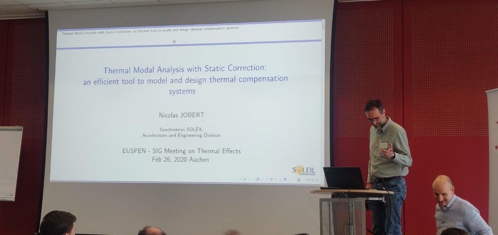
Contribution to EUSPEN 2020 – SIG Meeting on thermal effects

Well, it doesn’t look like much but those two guys on the picture are smiling. And how do we know that? Because they are not wearing a mask! In public! Ah, those were the days …

On this occasion, I presented a simple addition to the modal method for creating compact – though accurate – state space models for mechanical systems submitted to thermal disturbances.

Then, I applied it to a synchrotron light source primary mirror. This is a typical case where the figure of merit (here: slope error) is dominated by the local, quasi-static response (here: bump) which would be grossly underestimated when not including static correction. I also show that the brute-force approach (including hundreds of modes) would very slowly converge to a … very inaccurate value. The presentation can be downloaded here:

This abstract is archived on the EUSPEN repository under number 1219030602.

For those interested, you can reach me using the contact form.

Happy model reduction!